Bringing it all together with GitLab CI

Note: This post is part of a series on reproducibility. With any luck, it will make sense on its own. But it may be helpful to start from the beginning.

Up to this point, we’ve talked about a lot of different tools and ideas, and how they fit together to make analyses reproducible. In the last post, I went over how we can use Docker to make it easier to share your working environment to facilitate transparency and reproducibility. But even with these tools, the process of getting someone to the point where they can actually run your analysis and look at the results is still somewhat involved. At the very least requires them to download your analysis code and a Docker image to their own computer, which is likely to be a fairly high hurdle for many folks.

Since the goal of this whole series is eliminating the friction of sharing and re-running analyses, what I want to talk about in this post is how to knock down these last barriers to make your analysis accessible to even the most casual and technically-challenged observer. This is going to involve Docker, git and GitLab’s incredibly useful (and free!) continuous integration tools.

What is continuous integration?

In this section, I’m going to briefly outline the ideas and tools underlying continuous integration. I’m going to talk a bit about git and version control here, but nothing we’re going to discuss in this post will require you to interact with the command-line version of git.

I am not a git master by any stretch of the imagination (I get by with a working knowledge of commit, push, pull and merge) and you don’t need to be either to make this work for you. It will, however, be helpful to be familiar with the basic ideas. And a basic understanding of git and other version control systems should really be considered a life skill for quantiative epidemiologists, social scientists, etc. at this point anyway.

Continuous integration (CI) is an approach to software engineering that emphasizes testing your code after every meaningful change to the code base. These tests can take many forms, but the one we’re going to focus on is whether your project is able to successfully build, i.e. generate whatever targets you need. In software engineering, this often means that we have successfully generated an executable file that can then be run. In our toy Gaussian mixture model example, we’re going to consider a successful build to be one in which the PDF showing our model inputs and results is successfully generated.

One of the key advantages of working on GitLab (as compared to GitHub) is that GitLab has CI functionality baked in, rather than necessitating external tools. But beyond this, GitLab provides access to free cloud computing to run your tests. What this means is that anyone can make a copy of our project, make a change to the input parameters and re-build everything to see if it still works under different conditions.

Because GitLab (like GitHub and Bitbucket, another great free source-code hosting site) allows you to make changes to code and data directly through its website, it is not necessary to download the code to your computer to make changes, eliminating a major barrier to getting other people to interface with your code and results.

So, for the remainder of this post I’m going to talk about how I set up the toy model project to use Gitlab’s CI functionality and then give a step-by-step example of how to make a copy of the repository and make changes to it, all through GitLab’s web interface.

Setting up GitLab CI

Getting GitLab’s CI up and running for this project turns out to be very simple and to mimic the process of running it locally. To accomplish this, we tell GitLab CI what Docker image we want to use to create the environment to run our analysis in, what code to run, and what output files we want to be returned to us when it’s done.

To tell the CI system what to do, we create a YAML file called .gitlab-ci.yml and put it in the root of the reproducible-stan repository. YAML (which Wikipedia informs us is a recursive acronym for “YAML Ain’t Markup Language”, because, well, why not) is just a way of storing structured data (think of an R list with named fields or a Python dictionary) in plain text. Here’s the YAML file for running the toy model:

image: jonzelner/rstan:latest

pdf:
  script:
    - make pdf
  artifacts:
    paths:
      - output

The first line tells GitLab that we’re going to be running everything within the jonzelner/rstan image we talked about in the last post.

The field script: under pdf: tells GitLab to run the command make pdf as our test (i.e., run everything and generate the PDF output). The information listed under the field artifacts: tells GitLab what directories or files to save after running the tests. In this case, we tell it to keep everything in the output directory. This includes the final PDF as well as all of the individual PDF files for the figures and output from the Stan model.

Making changes

Ok - we’re going to go step-by-step through the process of making a copy of the repository holding the toy model project, making changes, and looking at the results. If you don’t have a GitLab account, the first thing to do is to go here and make one.

Fork the project

Once you’re up and running with GitLab and logged into your account, head over to the project page. At the top of the page, you should see something like this:

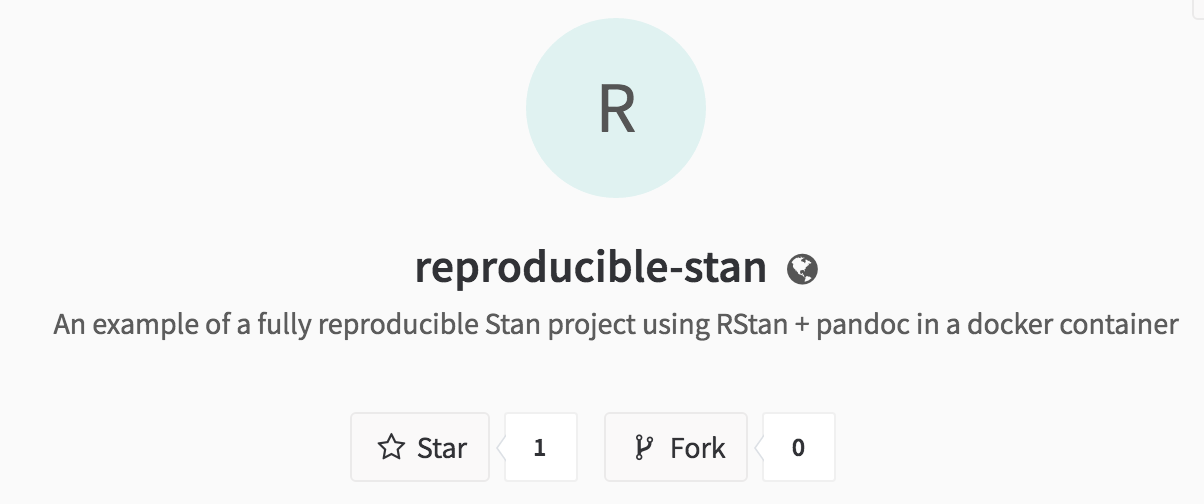
To copy the project into your own workspace click on “Fork” and follow the directions that come up. For more information on forking projects on GitLab, check this out.

Modify the data and re-run the analysis

Everything from here on out will assume you’ve successfully forked the project into your own GitLab workspace and are working from inside the forked project.

So, once you’ve done that, use the toolbar on the left-hand side to click on “Files”, which will show you all the files associated with the project:

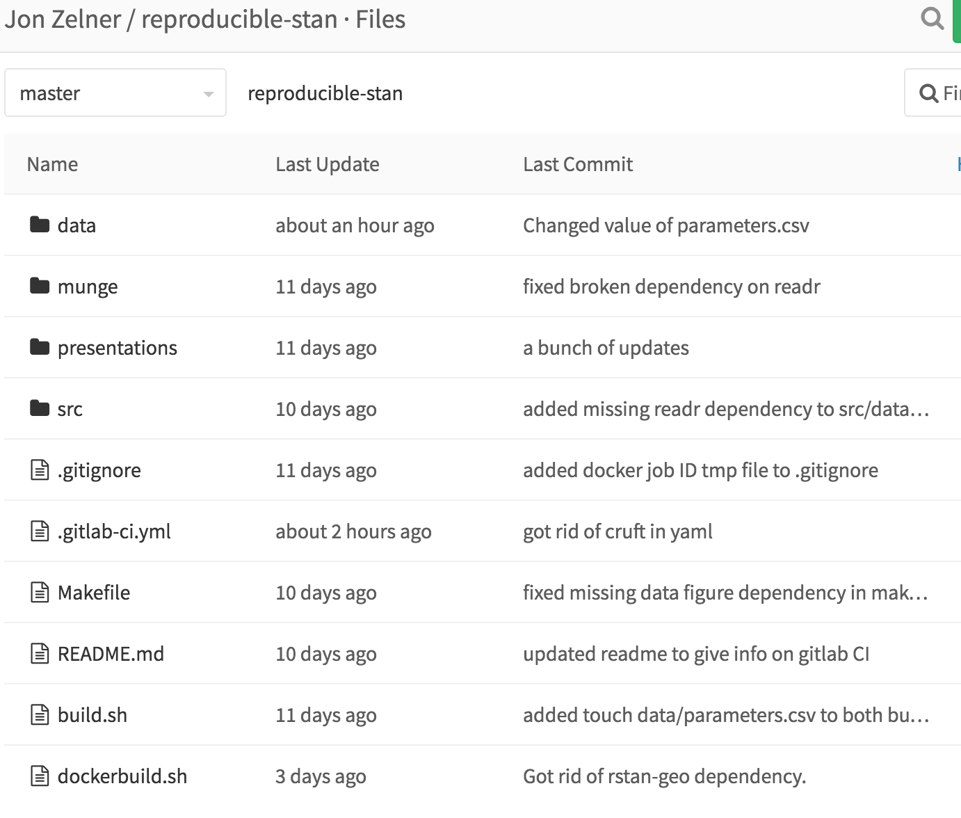
From this window, click on “data”, and then within data, click on “parameters.csv” to open up the input data. You should see this:

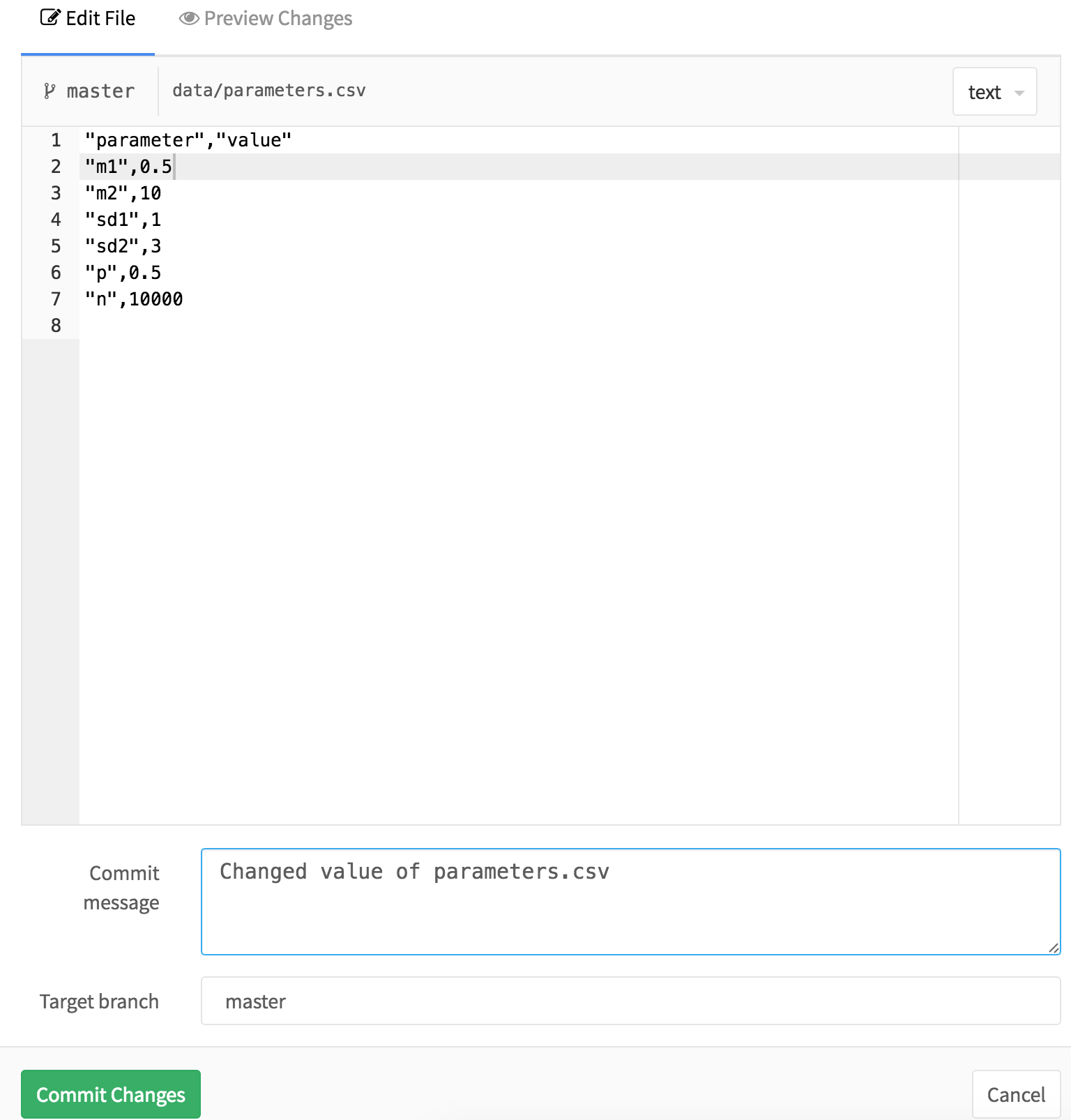
In this file, you can modify the input data. In this case, let’s change the mean of the first component to 0.5 from 2. You can say what you did and why in the “Commit message” field if you want to save a detailed record of what you did. To save your changes, click the big green “Commit” button at the bottom of the screen.

This is where the CI system kicks in! After you hit commit, it reads the contents of .gitlab-ci.yml and launches a computing instance with the docker image jonzelner/rstan on it. To see the status of the build, you can use the navigation bar on the left and click “Builds”. At the top, you’ll see something like this:

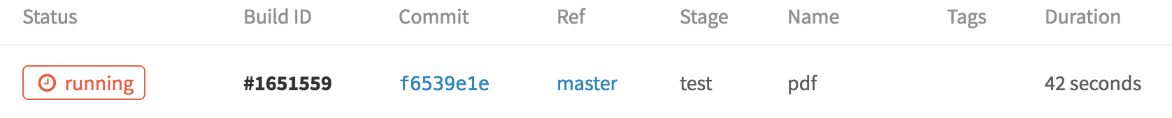
This just tells us that the build is still running, of course. It will take a few minutes because the server has to pull the Docker image, which is currently on the large side at around 5GB. But once it’s done, this screen will look like this:

Check out the results

Now that everything has finished running, we can download and inspect the results by clicking on the download icon to the right of the build status:

This will download a file called artifacts.zip that includes all of the output from the model. To see what’s in the file without running, forking, etc, click here.

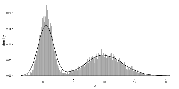
Ok - so here’s what the new simulated data look like:

And here’s how the posterior distribution of the parameter mu1 is compares to the new value of 0.5 (represented by the dashed vertical line):

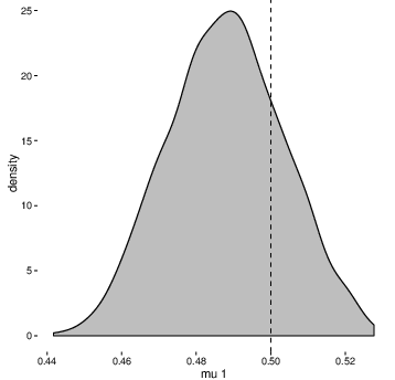
Not bad, especially for basically zero effort (and expense)!

Conclusion

So, hopefully this now gives a sense of how we can make the most use of Docker to make it almost painless for other people to examine and replicate results. The example I talked about today - just modifying a single parameter in a single file - is deliberately simplistic (although it may be very useful in many cases, for example examining how the results of an agent-based model change as the result of modifying a key parameter).

If you wanted to do something more involved, like changing the underlying model code (in src/model.stan), it would probably be most expedient to clone the reproducible-stan repository to your laptop, make changes, and then push those back to your forked repository on GitLab. This requires some work, but it really isn’t very hard and the benefits are enormous! If you’re not comfortable working on the command line with git, there are GUI git clients out there, like SourceTree that make it a bit easier.

Another thing that I hope this series of posts showcases is the advantage of working with free and open-source software (FOSS). If R and Stan weren’t FOSS, we couldn’t easily package them up in a publicly available Docker container for anyone to use! I try to remain non-partisan in the pointless R/Stata/SAS wars, because I think whatever makes you productive is probably what you should be using. For me, that’s R, both because I prefer the language (despite its peculiarities and unnecessary frills) and because the fact that it is free and open-source means that the possibilities for sharing and extending the language (for non-commercial purposes at least) are nearly endless!

That brings this initial series on reproducibility to a close for now. In future posts, I hope to talk a bit more about the issues that complicate reproducibility (e.g. sharing projects built on proprietary or sensitive data) and some more advanced tricks, like using GitHub CI to deploy your results to a free-standing web site.

Let me know what you think of all these posts and what else you might like to see at jon at jonzelner.net!

Previous: It’s not reproducible if it only runs on your laptop.